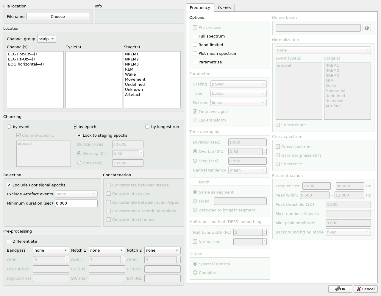
Analysis console

Wonambi’s analysis console allows the flexible selection of signal for a variety of analyses, including frequency domain analyses and phase-amplitude coupling (PAC).

The console is read from left to right. On the left-hand half of the console is the signal selection pane. Signal can be selected by event, epoch or longest run, and by channel, cycle and stage, with flexible concatenation options, and with artefacted signal exclusion.

On the right-hand half is the analysis pane, arranged into 3 tabs: Frequency, PAC and Events. You may apply any or all of these analyses at once by activating them in each tab.

To open the dialog, click on Analysis -> Analysis console.

File location

Select the base name and location of the data files. The analysis console creates CSV files containing the raw analysis data, with suffixes for each analysis type:

• _freq: Frequency

• _pac: PAC

• _evtdat: Events

• _fooof: Spectral parametrization report

Note

These data files can become quite large depending on the analysis.

Chunking

Different analyses require different lengths of signal, hence the chunking option. You may chunk by event, epoch or longest run.

Chunking by event gathers all events of the type(s) selected as individual segments. If you wish to gather only the signal for the channel on which an event was marked, keep the Channel-specific box checked. Alternatively, you may wish to gather signal concurrent to an event on all selected channels. In this case uncheck Channel-specific.

Note

Channel-specific will only gather events marked on the specified channels. If unchecked, all events of the specified types will be gathered, including those marked on channels other than those specified, and including “orphan” events with no associated channel.

Chunking by epoch gathers all relevant signal cut up into segments of equal duration. To obtain the epochs as segmented by the Annotation File for sleep scoring, check Lock to staging epochs. Alternatively, you may select a different epoch length with Duration (sec). In this case, all relevant signal, after the specified concatenation, will be segmented at that duration, starting at the first sample of relevant signal. Any remainder is discarded. Discontinuous signal concatenation is unavailable with this option. You may also set an overlap between consecutive segments, using Overlap or Step. Overlap is expressed as a ratio of duration, between 0 and 1. Step sets the distance in seconds between each consecutive segment.

Chunking by longest run gathers all relevant signal cut up into the longest continuous (uninterrupted) segments. For example, if in the sleep cycle selected there is a run of 10 minutes of REM, with another isolated 30s epoch of REM cut off from the rest, this option will return two segments, one 10 minutes long and one 30s long.

Location

Next, you will see Channel group and Channel(s). You may select signal from several channels within a same group.

If you have delimited cycles (see Annotations), the cycle indices will appear under Cycle(s). You may select one or several cycles in which to find epochs or events. If no cycle is selected, data selection will ignore cycles.

You may also select one or several Stage(s) in which to find epochs or events. If no stage is selected, data selection will ignore stages.

Rejection

Exclude Poor signal epochs removes epochs marked as Poor signal.

Exclude Artefact events removes signal concurrent with Artefact events on all channels.

Minimum duration (sec) sets the minimum length of segments after artefact rejection and concatenation, below which the segment is excluded.

For Poor signal and Artefact event marking, see Annotations.

Concatenation

You can concatenate different stages, cycles, event types or channels. Discontinuous signal will only be concatenated if the Concatenate discontinuous signal box is checked. This holds for signal discontinuities introduced by artefact rejection.

Channel concatenation is only available if discontinuous signal is concatenated. Discontinuous signal concatenation is not available for by epoch chunking. Concatenation is not available when the Lock to staging epochs option is selected.

Info

This box dynamically displays the number of segments relevant to your data selection.

A segment is a slice of signal in time. It may contain data from one or several channels. Each channel in a segment is analyzed independently, and is represented by one row in the CSV output. For example, if you have 30 segments over 3 channels, the CSV output will have 90 rows.

Pre-processing

You may apply any or all of the following transformations to the signal before running the analyses on the right-hand side of the console. The selected transformations are applied in the order displayed.

• Remove 1/f: Removes the signal’s 1/f background activity, which can help bring out spectral peaks in the signal, above and beyond background activity. In Wonambi’s implementation, this is achieved by subtracting each signal sample from the next sample, effectively resulting in a ‘change’ signal.

• Bandpass: You may apply a variety of bandpass filter types with the drop-down menu, with options for filter Order, Lowcut and Highcut. You may instead choose to only apply a lowpass or highpass filter; in this case, only type in the Highcut or Lowcut, respectively.

• Notch: You may apply up to two notch filters (a.k.a. powerline filters). To do so, select a filter-type in the drop-down menu and enter the Order, Centre frequency and Bandwidth. Frequencies between (centre frequency +/- (bandwidth / 2)) will be attenuated.

Frequency

Wonambi offers a highly-customizable range of frequency domain transformations. For an in-depth discussion of the tools, see Analysis/Frequency Domain.

To activate frequency domain analysis, check Compute frequency domain. To apply the selected pre-processing before the frequency domain analysis, check Pre-process. To obtain a summary spectral plot, averaging all segments and channels, check Plot mean spectrum. To obtain a parametrization of the periodic components of the signal using the FOOOF algorithm (Haller et al., 2018), check Parametrize.

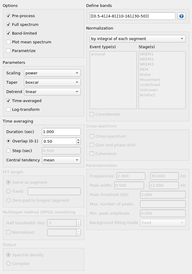
Options

This box controls the data export options, as well as pre-processing.

Pre-process: if checked, the raw data will be processed according to the options selected in the Pre-processing box, before frequency analyses are applied.

Full-spectrum: if checked, the full frequency spectrum will be exported in CSV format, with the suffix ‘_freq.csv’. Rows are segments and columns are sample frequencies from 0 to the Nyquist frequency.

Band-limited: if checked, band-limited power will be computed for the bands specified in the Define bands box. results will be exported in CSV format, with the suffix ‘_band.csv’. Rows are segments and columns are bands.

Plot mean spectrum: if checked, a summary spectral plot will be displayed, averaging all segments.

Parametrize: if checked, the resulting spectrum will be analyzed using the FOOOF algorithm (Haller et al., 2018). Results will be exported to CSV format, with the suffix ‘_fooof.csv’.

Note

The full spectrum, mean spectrum plot and FOOOF parametrization can only be obtained if each transformed segment has the same number of frequency bins, i.e. the same frequency granularity. Frequency granularity is set by the FFT length, which in a simple periodogram is equal to the segment length. As a result, it is not possible to obtain the mean of a simple periodogram if the input segments vary in length, as would likely be the case if analyzing events or longest runs. There are a few workarounds:

1. Use a Time-averaged periodogram, a.k.a. Welch’s method; in this case, FFT length is set by the time window Duration. However, time-averaging is impractical for short data segments such as spindles.

2. Set a Fixed FFT length; in this case, shorter segments will be zero-padded to the FFT length, but longer segments will be truncated (not recommended).

3. Use Zero-pad to longest segment to set FFT length to the longest segment and zero-pad all shorter ones. This option is recommended for short data segments such as spindles.

Parameters

Scaling sets the type of frequency domain transformation. To obtain the power spectral density (PSD), set Scaling to ‘power’. For the energy spectral density (ESD), set it to ‘energy’. The ‘fieldtrip’ and ‘chronux’ type transformations are also provided, but note that these may violate Parseval’s theorem.

Taper sets the type of tapering function (a.k.a. windowing function) to use. Commonly used tapers are ‘boxcar’, ‘hann’ and ‘dpss’ (see below for ‘dpss’).

Detrend sets the type of detrending to apply: ‘linear’, ‘constant’ or ‘none’.

If Time-averaged is checked, the data will be windowed according to the parameters in the Time averaging box. Time averaging is used in Bartlett’s method and the closely related Welch’s method.

Time averaging

This box is activated by the Time-averaged checkbox in the Parameters box. It controls the length and spacing of the time windows.

You must set a Duration, in seconds, and either an Overlap or Step. Overlap is expressed as a ratio of Duration, between 0 and 1. An Overlap greater than 0 is equivalent to Welch’s method; at 0 it is equivalent to Bartlett’s method. Alternatively, you may use Step to set the distance in seconds between each consecutive window.

FFT length

This box sets the window length for the Fourier transform. An FFT length that is Same as segment is best for most purposes.

But in cases where you want to, for instance, average the spectra of data segments of varying lengths, you may want to set a fixed FFT length. To do this, you may either set it manually with Fixed or automatically with Zero-pad to longest segment. In the latter case, the FFT length is set to the length of the longest segment N, and zeros are added to the end of all shorter segments until they reach length N. Zero-padding is a computationally efficient way to effectively interpolate a coarse-grained frequency spectrum to a finer grain.

Multitaper (DPSS) smoothing

This box is activated if ‘dpss’ is selected as Taper in the Parameters box. Here you can set the smoothing parameters for the DPSS/Multitaper method.

Half bandwidth sets the frequency smoothing from - half bandwidth to + half bandwidth.

You may normalize the halfbandwidth with Normalized (NW = halfbandwidth * duration). The number of DPSS tapers is then 2 * NW - 1.

Define bands

This box is activated by the Band-limited checkbox in Options.

You may enter bands of interest in either list or dynamic notation.

List notation: [[f1,f2],[f3,f4],[f5,f6],…,[fn,fm]]

e.g. [[0.5-4],[4-8],[10-16],[50-100]]

Dynamic notation: (start, stop, width, step)

e.g. (35, 56, 10, 5), equivalent to [[30-40],[35-45],[40-50],[45-55],[50-60]] in list notation.

Note that ‘start’ and ‘stop’ are centre frequencies. Also note that ‘start’ is inclusive, while ‘stop’ is exclusive.

Output

Use this box to select a Spectral density output or a Complex output.

Normalization

You may normalize the resulting spectral data, either with respect to its own integral or with respect to a normalization period. When normalizing with respect to a normalization period, the selected frequency analyses are applied directly to the normalization period signal.

To normalize a signal to its integral, select by integral of each segment in the drop-down menu. Each power value will then be divided by the average of all power values for that segment.

To normalize with respect to a normalization period, you must first demarcate this period, either using Event Type(s) or Stage(s). For example, you may have recorded a quiet wakefulness period at the start of the recording. In this case, you may create a new Event Type and call it something like ‘qwak’ and mark the entire period as an event on the trace. You may need to increase the Window Length (in View or on the toolbar) in order to mark the entire period within one window.

Note

In Wonambi, events are channel-specific by default, but for the purposes of demarcating a normalization period, you may mark events on any channel in the channel group. Just make sure the channel is still in the channel group at the moment of analysis.

Once the normalization period is marked as one or several ‘qwak’ events, select by mean of event type(s) in the drop-down menu and select ‘qwak’ in the Event type(s) list. The power values for each segment will then be divided by the mean power values of all ‘qwak’ events.

Alternatively, you may want to normalize with respect to a stage mean. In this case, select by mean of stage(s) and select the desired stage(s) in the Stage(s) list. The power values for each segment will then be divided by the mean power values for all 30-s epochs of the selected stage(s).

Warning

Normalizing by stage(s) may extend processing time considerably.

For event type and stage normalization, you may choose to concatenate all relevant normalization periods before applying the frequency transformation, instead of first applying the transformation and then averaging. To do this, check Concatenate.

Note

Like the mean spectral plot, normalization is only available if each segment has the same frequency granularity. See the note about frequency granularity above.

Parametrization

Wonambi allows parametrization of power spectra using the FOOOF algorithm:

Haller M, Donoghue T, Peterson E, Varma P, Sebastian P, Gao R, Noto T, Knight RT, Shestyuk A, Voytek B (2018) Parameterizing Neural Power Spectra. bioRxiv, 299859. doi: https://doi.org/10.1101/299859

From the FOOOF Github page:

FOOOF is a fast, efficient, physiologically-informed model to parameterize neural power spectra, characterizing both the 1/f background, and overlying peaks (putative oscillations).

The model conceives of the neural power spectrum as consisting of two distinct functional processes:

• A 1/f background, modeled with an exponential fit, with:

• Band-limited peaks rising above this background (modeled as Gaussians).

With regards to examing peaks in the frequency domain, as putative oscillations, the benefit of the FOOOF approach is that these peaks are characterized in terms of their specific center frequency, amplitude and bandwidth without requiring predefining specific bands of interest. In particular, it separates these peaks from a dynamic, and independently interesting 1/f background.

If selected, the algorithm will create a CSV report:

You may adjust the following parameters:

• Min. frequency and Max. frequency: set the frequency range across which to model the spectrum.

• Peak threshold: sets a threshold above which a peak amplitude must cross to be included in the model. This parameter is in terms of standard deviation above the noise of the flattened spectrum.

• Max. number of peaks: sets the maximum number of peaks to fit (in decreasing order of amplitude).

• Min. peak amplitude: sets an absolute limit on the minimum amplitude (above background) for any extracted peak.

• Min. peak width and Max. peak width: set the possible lower- and upper-bounds for the fitted peak widths.

• Background fitting mode: ‘knee’ allows for modelling bends, or knees, in the aperioic signal that are present in broad frequency ranges, especially in intracranial recordings. ‘fixed’ models with a zero knee parameter.

Phase-amplitude coupling (PAC)

Wonambi’s analysis console offers a phase-amplitude coupling analysis (PAC) GUI that ports directly to the Tensorpac package, by Etienne Combrisson.

In order to compute PAC, you must first install tensorpac from the command line (PC) or terminal (Mac):

pip install tensorpac

In the analysis console, select Compute PAC to enable PAC analysis, and select Pre-process to apply the selected pre-processing transformations before analysis.

Choose a PAC metric in the drop-down menu.

You may enter one or several phase and amplitude frequencies. Band limits should be separated by a hyphen ‘-’, and each band enclosed in square brackets ‘[]’, separated by commas ‘,’. The entirte epression should also be enclosed in square brackets.

For example, to detect coupling between delta (0.5-4 Hz) and theta (4-8 Hz) as phase frequencies, and low gamma (LG; 30-60 Hz) and high gamma (HG; 60-120 Hz) as amplitude frequencies, you would enter:

[[0.5-4],[4-8]] for Phase frequencies, and

[[30-60],[60-120]] for Amplitude frequencies.

This will yield 4 PAC values per segments: delta-LG, delta-HG, theta-LG and theta-HG PAC.

Alternatively, you may use dynamic notation in this format: (start, stop, width, step).

For example, to get the range of amplitude bands between 30 Hz and 130 Hz in non-overlapping 20-Hz bands, you would enter:

(40,140,20,20).

Notice that start and stop are centre frequencies. Notice also that start is inclusive but stop is exclusive, so in order to capture 110-130 Hz, stop must be set after the centre frequency, i.e. 121-140.

For more information, see the Tensorpac documentation.

Events

The console’s Events tab allows the extraction of a suite of commonly studied parameters. Event parameters are divided into global parameters, local parameters and slow wave parameters.

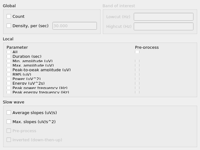
Global

• Count simply returns the number of segments.

• Density, per returns the number of segments divided by the number of epochs of relevant signal. The relevant signal is all epochs corresponding to the cycle(s) and stage(s) selected in the Location box. You may set the epoch length in seconds with the text box.

Band of interest

For Power, Energy, Peak power frequency and Peak energy frequency, you may set a band of interest. These analyses are then carried out only over that spectral band. If no frequencies are specified, analyses are applied to the entire spectrum.

Local

For each parameter, check the box next to it to extract it, and select the corresponding box in the Pre-process column in order to apply the selected pre-processing before analysis. Note that for all parameters except Duration, the output will contain one value per channel per segment.

• Duration: The segment duration, in seconds.

• Min. amplitude: The lowest amplitude value in the signal.

• Max. amplitude: The highest amplitude value in the signal.

• Peak-to-peak amplitude: The absolute difference between the lowest and highest amplitude values in the signal.

• RMS: The square root of the mean of the squares of each amplitude value in the signal.

• Power: The average power (from a simple periodogram) of the signal over the band of interest. Best used for stationary signals.

• Energy: The average energy (from a simple periodogram) of the signal over the band of interest. Best used for signals with a clear beginning and end, i.e. events.

• Peak power frequency: The frequency corresponding to the highest power value in the band of interest.

• Peak energy frequency: The frequency corresponding to the highest energy value in the band of interest.

Slow wave

These are local parameters that apply only to slow waves. You may still apply these analyses to any signal, but if the signal does not have the morphological characteristics of a slow wave, the output will be nan (not a number).

Average slopes and Max. slopes each return 5 values: one per slow wave quadrant and a fifth for the combination of quadrants 2 and 3:

• Q1: First zero-crossing to negative trough

• Q2: Negative trough to second zero-crossing

• Q3: Second zero-crossing to positive peak

• Q4: Positive peak to third zero-crossing

• Q23: Negative trough to positive peak.

Average slopes is the amplitude difference between the quadrant start and end divided by the quadrant duration, in μV/s.

Max. slopes is the maximum value of the derivative of the smoothed signal (50-ms moving average) of the quadrant, in μV/s².